Citation:

Frenz, B., Walls, A., Egelman, E. et al. RosettaES: a sampling strategy enabling automated interpretation of difficult cryo-EM maps. Nat Methods 14, 797–800 (2017). https://doi-org.offcampus.lib.washington.edu/10.1038/nmeth.4340
While the previous workflows have address model building and model refinement, none of the aforementioned tools deal with completion of large segments of protein. These may arise in several cases:
- Homology models (particularly distant ones) may have large insertions, or even entire domains that are lacking.
- The models produced from
denovo_densitymay be missing significant fractions of the backbone - It may be difficult to manually trace long stretches of low local resolution into density
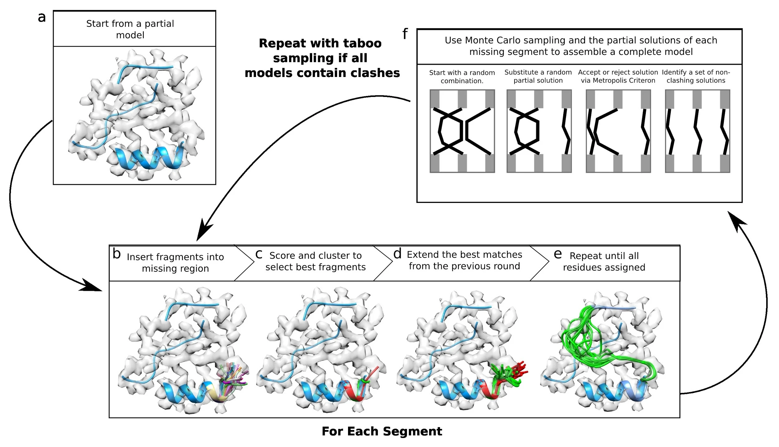
To address these issues, we have developed a tool called Rosetta Enumerative Sampling, which uses a
ensemble search algorithm to determine a large number of conformations that are both consistent with the
density and the Rosetta energy function. This tool can be used on a partial models from the denovo_denisty
application, an incomplete homology model, or any other starting structure. An overview of the method is
depicted in the image below:
RosettaES runs best when working with data at resolutions 5 Å or better with segments to rebuild shorter than 50 residues. However, with very large amounts of sampling (e.g., ensemble sizes > 250), reliable models may be produced with segments longer than 100 residues. At resolutions worse than 5 Å, this tool may be unreliable. The method can be used on both segmented and unsegmented density maps, however, removal of density belonging to parts of the structure not being modeled may improve results.
Running RosettaES model building consists of three main steps.
- A preparation step builds the fragments that are to be used in conformational sampling.
- A rebuilding step will identify each unassigned segment in the initial model and build an ensemble of possible solutions for each.
- A combination step finds all the consistent subsets of interactions, and refines all such models (if there is only one segment, the script simply refines all structures in the ensemble).
- In this combination step, if assembly fails to find a consistent set of solutions, an additional round of sampling will be carried out, forcing different solutions than the previous model.
Compared to the other sections, the workflow is a bit more complicated when extended to multiple compute
cores. To handle job distribution we have included a python script RunRosettaES.py that manages this job
distribution among available CPUs on a single machine. (The script is included as part of Rosetta, in
/main/source/scripts/python/public/EnumerativeSampling, as well as in this tutorial). For dealing with
job schedulers or clusters incompatible with this script, section 5E gives an overview of job distribution with
RosettaES.
Step 5A. Fragment Picking
The first step – much like Scenario 4 – involves selection of “fragment files,” which predict backbone
conformation from local sequence. Unlike Scenario 4, we have a custom algorithm for fragment picking.
These fragments will need to be generated before running RosettaES; the following command will generate
these files (5_rosettaES/A_PickFragments.sh):
#!/bin/bash

$ROSETTA3/source/bin/grower_prep.default.macosclangrelease \
    -pdb input.pdb \
    -in::file::fasta t20sA.fasta \
    -fragsizes 3 9 \
    -fragamounts 100 20 \
This will generate 100 3 residue fragments and 20 9 residue fragments, named 100.3mers and 20.9mers, that are then used in subsequent steps of the rebuilding process.
Step 5B. Generate Possible Conformations For Each Segment
The grower considers assigning positions for each unassigned segment of density (that is, each stretch of amino acids present in the fasta file but missing from the input structure). Each segment is referred to using a segment id, in which each segment is numbered from N- to C-terminus (with multiple chains given in order in the input fasta file). The script is run in two parts: first, the script is run once for each segment to rebuild; then, the script is run in “assembly mode” given the outputs produced by rebuilding each segment individually. Thus, for rebuilding the two segments in the test case, the script is called three times: once to build each segment, and once to assemble the results.
In the first step, we perform conformational sampling of each of the two segments, generating an ensemble
of putative solutions for each. This can be done calling the command (5_rosettaES/B1_SampleSegment1.sh):
#!/bin/bash

python $ROSETTA3/source/scripts/python/public/EnumerativeSampling/RunRosettaES.py \
    -rs runES.sh \
    -x RosettaES.xml \
    -f t20sA.fasta \
    -p input.pdb \
    -d T20S_48A_alpha_chainA.mrc \
    -l 1 \
    -c 16 \
    -n loop_1
The arguments to this program are as follows:
-rs runES.sh- the script that is launched on each core and contains Rosetta flags and inputs-x RosettaES.xml- the XML script describing parameters for conformational sampling (see below)-f t20sA.fasta- the input fasta file (with chainbreaks specified by ‘/’)-p input.pdb- the input pdb file. This needs to match the input sequence, and all residues present in the fasta but absent in the PDB will get built.-d T20S_48A_alpha_chainA.mrc- the input density map-l 1- the segment id of the segment to rebuild. This command should be called once for each segment to rebuild, varying this argument from 1 to N-c 16- the number of compute cores to use-n loop_1- the output tag for this job (results will be placed in a folder with this name). Tags should be unique for each segment.
The input XML file exposes key parameters for conformational sampling. In the tutorial, this file,
5_rosettaES/RosettaES.xml, contains a block:
...
  <FragmentExtension name="ext" fasta="t20sA.fasta" scorefxn="dens" censcorefxn="cendens"
      beamwidth="32" dumpbeam="0" samplesheets="1"
      read_from_file="0" comparatorrounds="100" continuous_weight="0.3" looporder="1"
      writelps="1" minmelt="15"
      readbeams="%%readbeams%%" storedbeams="%%beams%%" steps="%%steps%%" pcount="%%pcount%%"
      filterprevious="%%filterprevious%%" filterbeams="%%filterbeams%%">
    <Fragments fragfile="100.3mers"/>
    <Fragments fragfile="20.9mers"/>
  </FragmentExtension>
...
The sampling behavior of RosettaES is controlled by the block above. Many of the tags in this block –
looporderdumpbeamread_from_filestoredbeamsstepspcountfilterpreviouscomparitorrounds- and
filterbeams
– are used by the job distribution script to pass results from one step to the next, and they should be left as-is. Others are user-specified, and can be modified based on the size of the loop and resolution of the data:
beamwidth: controls the maximum number of solutions to be held at each step. Setting the value higher will increase run time but may improve accuracy.- If you find 32 is not enough, we often use 256 for modeling more difficult regions
windowdensweight: the relative contribution of density in model selectionminmelt: how many residues previous (or after depending on the direction of fragment extension) to minimize before adding a residue.- WARNING If you are confident in your starting model, set this to 2-3, if it is from De-novo modeling leave it at 15
For many cases, the default parameters are sufficient. However, if the segment to grow is long (50+
residues), you may need to increase beamwidth; if the density is low resolution, you might need to decrease
windowdensweight to 15 or 20.
Several options should rarely be modified, but may need to be in specific cases:
samplesheets: Controls whether or not beta sheet sampling should be performed. It is recommended to use this except when working with symmetric systems.continuous_weight: Controls the penalty on discontinuous density.- Setting this value to 1 will completely remove any penalty on discontinuous density;
- setting it closer to 0 will increase the penalty. You may wish to raise this value to 0.7 (or more) if you anticipate the segment you are trying to model does not follow a continuous path of density.
Finally, the option comparitorrounds is used in multi-segment assembly (see section 5C)
After running the script with this XML, there are two important intermediate output files, placed in the folder
loop_1 (the argument to -n):
.lps(for loop partial solution) files, which are then combined in step 5C, in cases where there are multiple segments to modeltaboo/beamX.txtfiles, where X corresponds to the number of residues added to the segment. These are generated as the search adds residues, and are used to pass information from one step to the next (as additional residues are added in a single segment).
Note: This process should then be repeated for all remaining segments to rebuild In the tutorial, the
command 5_rosettaES/B2_SampleSegment2.sh builds conformations for the second segment in this file. All
segments can be sampled independently of one another, so if many compute nodes are available, each
segment can be sampled simultaneously on separate nodes.
Finally, while in most cases, users will want to take these models into the assembly step (part 5C), if there is
only one segment to rebuild, or if the sampling results want to be inspected, the final output ensemble can be
saved as PDB files with the command (5_rosettaES/B1.2_InspectIntermediates.sh):
#!/bin/bash

python $ROSETTA3/source/scripts/python/public/EnumerativeSampling/RunRosettaES.py\
    -rs runES.sh \
    -x RosettaES.xml \
    -f t20sA.fasta \
    -p input.pdb \
    -d T20S_48A_alpha_chainA.mrc \
    -l 1\
    -db loop_1/taboo/beam5.txt\
Note, the number of the beam file (17) corresponds to the total number of residues built. Intermediate results (after growing N residues) can be inspected by changing this to a lower number (e.g., beam14.txt shows solutions after 14 of the 17 residues have been rebuilt).
Step 5C. Find a set of consistent conformations.
In cases where there are multiple interacting segments, we want to find all nonclashing combinations. This
step will take the loop partial solution (lps) files generated in step B and use a Monte Carlo Assembly (MCA)
algorithm in order to identify sets of solutions that are self-consistent. This section assumes that all
missing segments have been built in step B. To run this assembly, we perform conformational sampling
using the script, passing the .lps files generated in step B (5_rosettaES/C_AssembleResults.sh):
#!/bin/bash

python $ROSETTA3/source/scripts/python/public/EnumerativeSampling/RunRosettaES.py\
    -x RosettaES.xml \
    -f t20sA.fasta \
    -p input.pdb \
    -d T20S_48A_alpha_chainA.mrc \
    -lps loop_*/lps*.txt
The flag -lps points to the outputs of the individual segment jobs’ output. As before, the script will use (and modify) an input XML file. For assembly, only a single parameter is important to modify: comparatorrounds=”100”. This parameter controls the number of Monte Carlo trajectories (it is unlikely you will need to change this parameter).
The output of this step is PDB files, that will be placed in the working directory with the prefix
aftercomparator_RRR_XXX.pdb, where RRR is the trajectory id, and XXX is the energy. A text file
recommendation.txt will be written that reports the clash score of the best model.
If the number in recommendation.txt is above +100 it is recommend you perform additional rounds of sampling. To do so, additional potential solutions should be sampled by repeating step B and providing the same directory name as input, without deleting the intermediate files. The script will then enter that directory and use the already-computed solutions (stored in the folder “taboo”) to guide sampling toward previously unexplored regions. See section D for more details.
If the number in recommendation.txt is below +100, then models should be run through Rosetta
refinement to accurately rank them. That can be done using this command (5_rosettaES/D_RefineOutput.sh):
#!/bin/bash

python $ROSETTA3/source/scripts/python/public/EnumerativeSampling/RunRosettaES.py\
    -f t20sA.fasta \
    -p input.pdb \
    -d T20S_48A_alpha_chainA.mrc \
    -c 16 \
    -rp aftercomparator_*.pdb \
    -rlxs runrelax.sh
Where runrelax.sh contains a command for relaxing structures in Rosetta.
Step 5D. Interpreting results
RosettaES will produce a 100 models as output (or whatever is specified in comparatorrounds), with scores in the file score.sc. When first looking at the output from a run, it is good to visually inspect the lowest- energy 5-10 structures. Ideally, these lowest-energy models will be very tightly converged, but the lack of convergence does not indicate failure in sampling, and the presence of convergence does not necessary indicate the solution is correct. Instead, the lowest-scoring models should be examined with attention to the following:
Insufficient sampling. Models should initially be inspected for clearly incorrect features that might not have been properly penalized by Rosetta. These include:
- unexplained density, particularly small sidechains placed into a large density protrusions
- regions with poor fit to density
- unresolved clashes
If these features are present in the lowest-energy models, it suggests that the conformational sampling performed by RosettaES may not have been sufficient. There are several ways to address this issue. The first is to increase conformational sampling. This can be done by either: a) increased the beamwidth parameter and rerunning anew, b) and/or performing additional rounds of taboo search (taboo sampling occurs automatically if the “taboo/” folder in the running directory is populated with beam files”), or c) reducing the search space by eliminating regions of density.
The latter can also be performed by manually removing parts of the map you do not wish to sample or by including additional portions of the model, for example if you are building a model that has 4 missing regions and you believe you have accurately sampled 3 of them (they do not posses any of the pathologies listed above and fit the density well), you can combine them by treating them as templates for RosettaCM (use a fasta file with the missing segment removed) and use the result as input for RosettaES to build the last region.
Unresolved residues. RosettaES will always attempt to build all residues present in the fasta file, however, in many cases not all residues will be resolved in the map (particularly at termini). Because RosettaES will heavily penalize models that do not fit the density, you will often find models that are “overly compacted” at termini or internal loops, to try to squeeze these residues into density.
If this happens at termini it is suggested that you examine intermediate structures that have yet to attempt to assign these unresolved residues in order to find a good model. If this happens internally (or if you have a good idea a priori what residues should be modeled), these regions can be removed from the input fasta. If internal segments are deleted, be sure to treat the deletion correctly, by putting a ‘/’ in the fasta file.
Step 5E. Customizing job distribution.
Job distribution in RosettaES is complicated, since each “growing step” can be parallelized, but subsequent steps need all the information from the previous step. Consequently, the script provided (RosettaES.py) manages jobs, by calling Rosetta jobs at each round, collecting and combining the results of the previous round, then splitting input files for the next round. On systems where it is not possible to run this script, this section describes in some detail what the script is doing.
To manage this the python script uses the provided XML file as input, rewriting several parameters depending on the protocol step. These varying parameters include:
readbeams, a boolean option that tells Rosetta whether it should load intermediate solutionsbeamfile, the name of the beamfile that stores the intermediate solutionssteps, how many residues to add (0 means only do filtering, otherwise set to 1, setting to “-1” will build all missing residues)pcount, used to uniquely tag output files from each corefilterprevious, a boolean option that controls whether intermediate solutions should be read for taboo searchfilterbeams, the filename of the intermediate solutions for use in taboo.
In order to build a missing segment the script will perform the following steps:
Launch a job with
- readbeams=”0”, beamfile=”na”, steps=”1”, pcount=”1”, filterprevious=”0”, filterbeams=”na”. This will produce a file named beam1.1.txt from Rosetta.
- Parse the beam1.1.txt file and split into N files (where N is the number of parallel jobs to run). New files are labeled beam_$r.$i.txt where $r is the number of residues added so far, and $i ranges from 1 to N.
- Submit N rosetta jobs with pcount set as the job number, readbeams set to “true”, and beamfile set to the corresponding output of step 2.
- Output files are parsed by the script and compiled into a single file with the name beam$r.txt, with $r the number of residues grown.
- Rosetta is run on a single core to filter the aggregate solution set. Here, readbeams=”1”, beamfile=”beam$r.txt”, and steps=”0”. A file named beam_0.txt will have the filtered results.
- Repeat steps 2-6 using the
beam_0.txtas the input for step 2. This is done until the segment is complete and Rosetta produces an empty file called finished.txt. The presence of this file triggers the program to perform one final round of filtering and exit.
The last step of RosettaES will additionally produce a file with the name lpsfile_$s.0.txt used for assembly.
To run assembly with these files first combine them into a single file, described below, and run with
readfromfile=”filename”. This new file should start with the a number corresponding to the total number of
missing segments, then for each missing segment provide a number for the total solutions in that segmented
followed by the solution information contained in the lpsfile_$s.0.txt described above. Segments should be
arranged to match the order in which they occur in the fasta.